Tutorial using Timeflux

This tutorial showcases the main mechanisms of HappyFeat, using Timeflux as a processing engine, and EEG data from the Physionet dataset, loaded using MNE.

Make sure to follow the steps in the Installation page first. Also, make sure Timeflux is installed in your environment:

python -m pip install timeflux
python -m pip install timeflux_dsp

Launching HappyFeat

If you installed from PyPI, launch HappyFeat using this command:

happyfeat

If you cloned the repository from github, the application's entry point is the Python script happyfeat_welcome.py. Navigate to the cloned repo and type the following:

python -m happyfeat.happyfeat_welcome

A "welcome" GUI opens, allowing you to create or load a workspace.

Creating and setting up a workspace

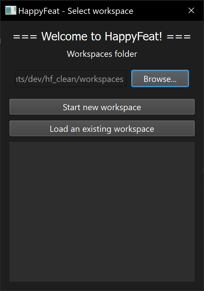
First, browse for the folder in which you would like HappyFeat to create and look for workspaces. This will be referred to as <workspaces>

Click on "Start new workspace" and enter a name for your workspace. This will be referred to as <newWorkspace>.

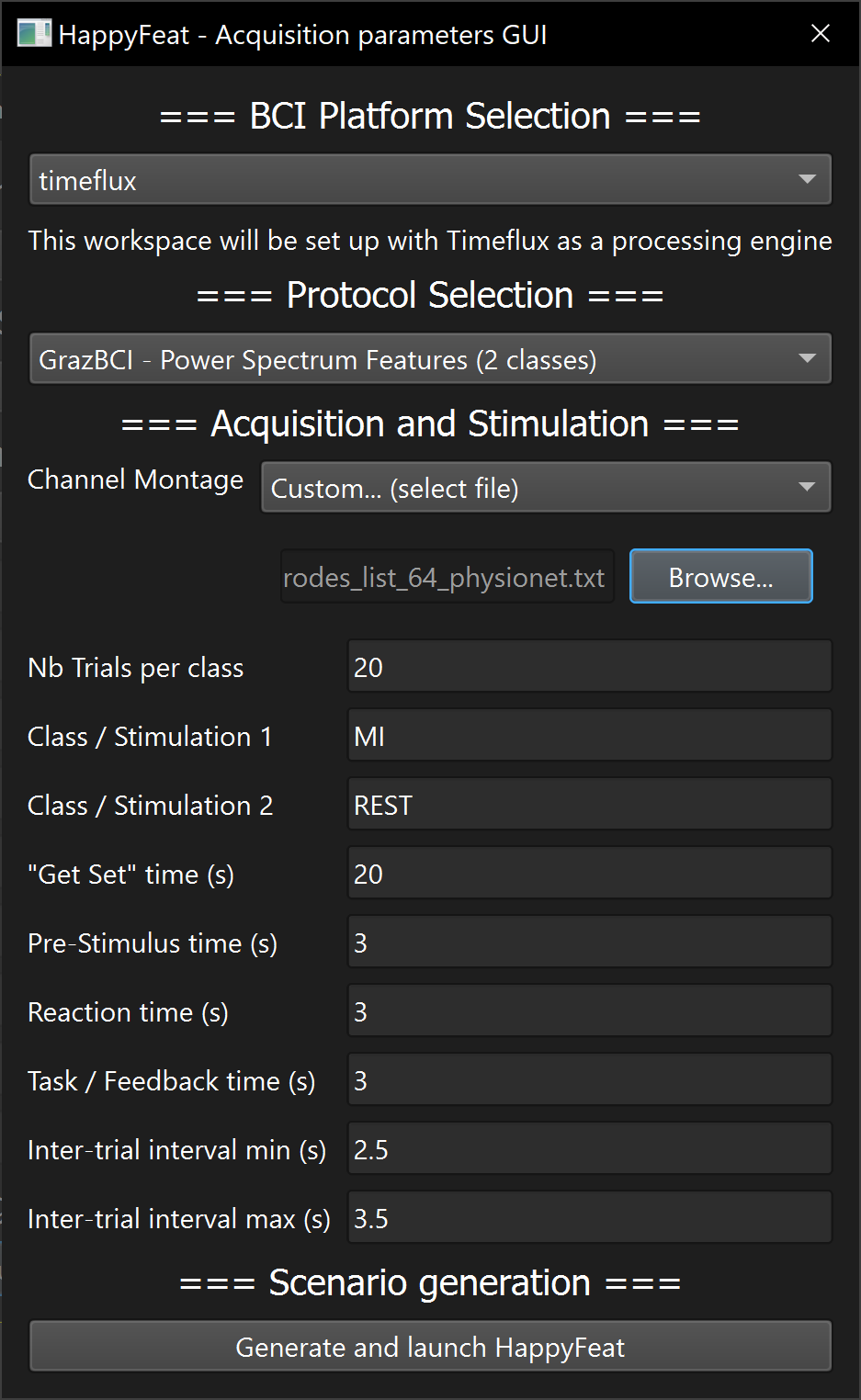
A new assistant GUI will open, allowing you to set up the BCI experiment parameters.

• In the first drop-down menu, select Timeflux as a BCI platform.

• In the second drop-down menu, select Graz BCI - Power Spectrum Features (2 Classes). This corresponds to the metric used in this workspace, and the associated data processing pipelines.

• In the Channel Montage drop-down menu, select Custom, then browse to select this file : <happyfeatInstallFolder>/tutorials/electrodes_list_64_physionet.txt

• You may leave the default values for the following parameters (nb trials per class, stimulation 1/2, etc.).

• Click on Generate and launch HappyFeat to proceed. The main GUI will appear.

Loading data from Physionet

In a terminal, navigate to HappyFeat's installation folder, then type:

python tutorials/physionetTutorial.py

This will download 3 EDF signal files to the folder: <happyfeatInstallFolder>/MNE-eegbci-data/files/eegmmidb/1.0.0

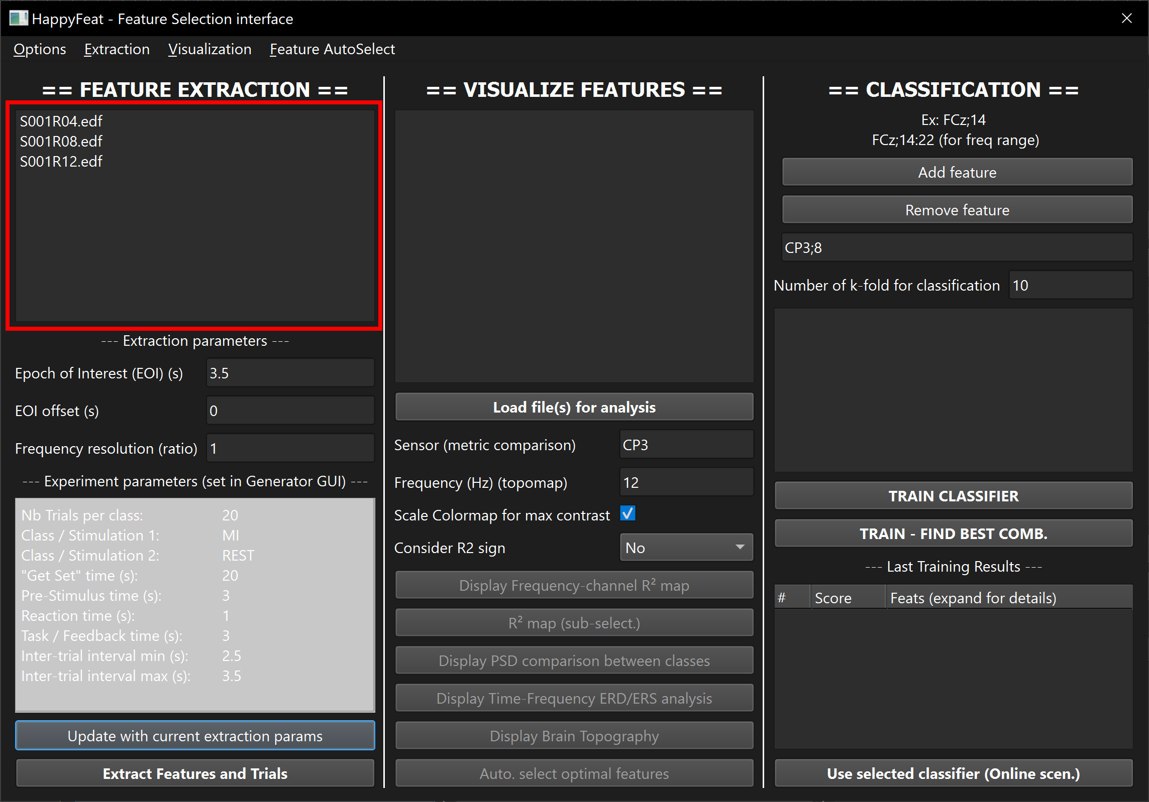
Copy those files to your new workspace's signals folder:

cp <happyfeatInstallFolder>/MNE-eegbci-data/files/eegmmidb/1.0.0/S001/*.edf <workspaces>/<newWorkspace>/signals

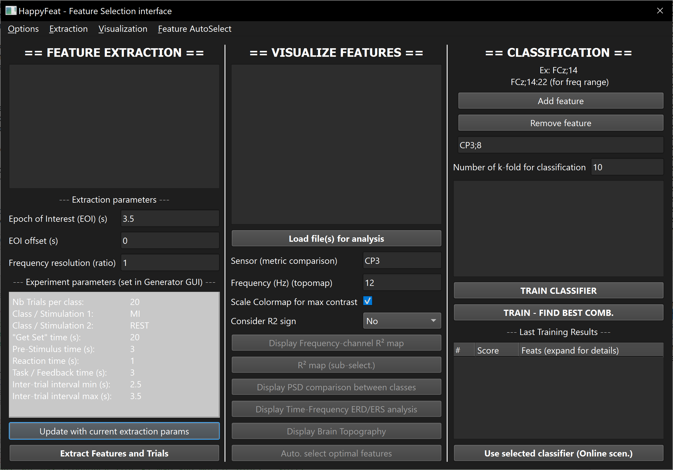
The files should appear in the list in the left panel of the application (Feature Extraction).

Extracting the features

Before extracting features from our EDF files, we still have a few more things to set up.

• Click on the Extraction menu in the top bar, and Set Class Stimulations. Enter T0;T2 and validate.

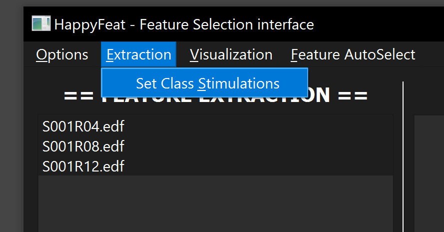
Note

Those are the trigger names in the EDF files for the Physionet dataset. T0 corresponds to the onset of a "Rest" trial, and T2 to a "imagine Right Hand movement" trial.

Since we have set this HappyFeat workspace to work with "MI" as Class 1 and "REST" as Class 2 (in the BCI pipeline setup GUI), we need to set the stimulations in the order T2;T0.

• Then, in the Extraction Parameters, set Epoch of Interest (EOI) (s) to 3, and leave the default values for other parameters.

• Select the 3 files in the list, and click Extract Features and trials. After a few seconds of processing, the extracted files should appear in the list in the central panel of the GUI.

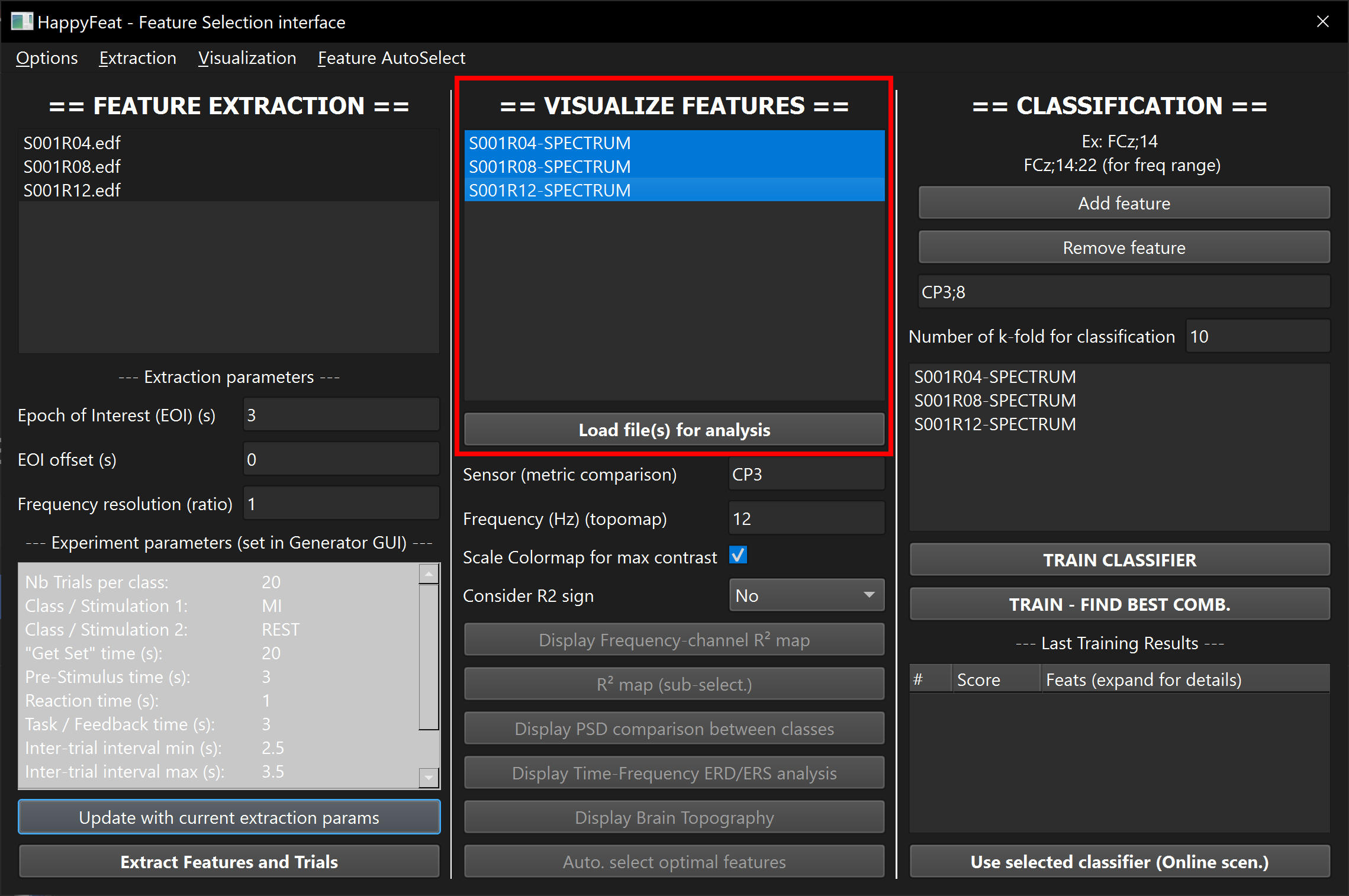
Visualizing metrics

Select the 3 "SPECTRUM" files in the list, and click on Load files for analysis, then on Display Frequency-channel R2 map. A browser window will open showing the discriminant power of the extracted metric (here Power Spectral Density), between Rest and MI, in terms of R2, over all trials of selected files.

Red squares are channel/frequency combinations with the best discriminant power.

To see things clearer, we can only consider channels of higher physiological significance, and narrow those results down to channels in the sensorimotor cortex and frequencies in the alpha & beta bands.

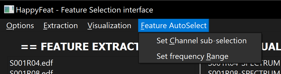
In the top menu, click on Feature AutoSelect then set the channel subselection to:

C5..;C3..;C1..;Cp5.;Cp3.;Cp1.;Fc5.;Fc3.;Fc1.;Cz..;Cpz.;Fcz.;C6..;C4..;C2..;Cp6.;Cp4.;Cp2.;Fc6.;Fc4.;Fc2.

... and the frequency range to 7:35.

Note

For the channel sub-selection, it's important to respect the (case-sensitive) original labels in the metadata of the recorded file. Hence the (not very practical) dots . and .. in the channel names above, coming from the Physionet dataset.

Now click on R2 map (sub-select.). A new browser will open, with a figure similar to the previous one, but showing only the requested sub-selection.

To visualize what happens in terms of frequencies for a given channel, enter C3.. (with the dots) in the Sensor for PSD Visualization field, then click on Display PSD comparison between classes. A new browser window will open, showing the average PSD of (accumulated) MI trials in red, and Rest trials in blue. The black curve shows the R2 value. This figure shows that for the sensor C3, we should be able to correctly discriminate between Rest and MI tasks by considering 12Hz

We can also visualize the projected topographic map of R2 values. Set Topographic freq to 12, and click on Display Brain Topography. A new (matplotlib) window is displayed, showing the topographic map, and high discrimation between the two tasks in Fc3 and Fc1.

Note

All figures are saved in the current workspace folder, in html or png format:

<workspaces>/<newWorkspace>/sessions/<sessionId>/figures/

Selecting features for training

There are now two ways forward for training the classifier:

• manually selecting the channel/frequency pairs, by entering them in the upper-right part of the GUI,

• or let HappyFeat automatically select the 3 "best" pairs (in terms of R2), in the previously configured subselections (i.e. sensorimotor cortex locations and in the alpha and beta bands).

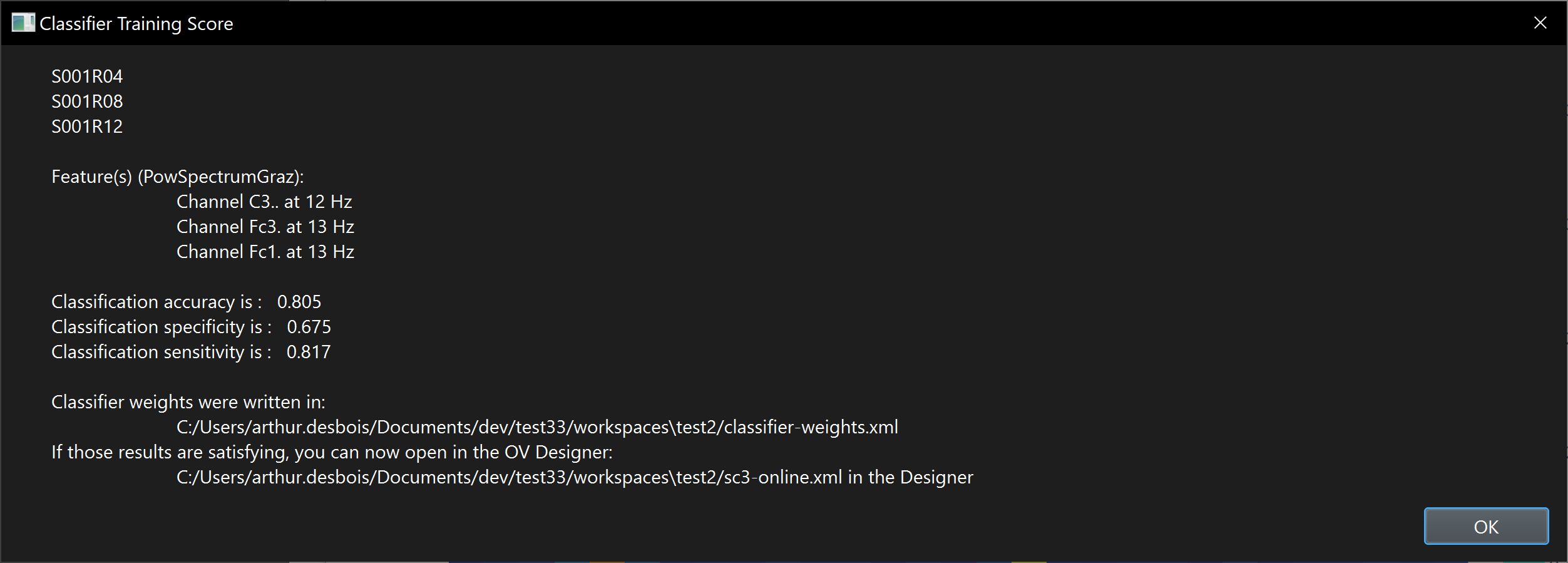
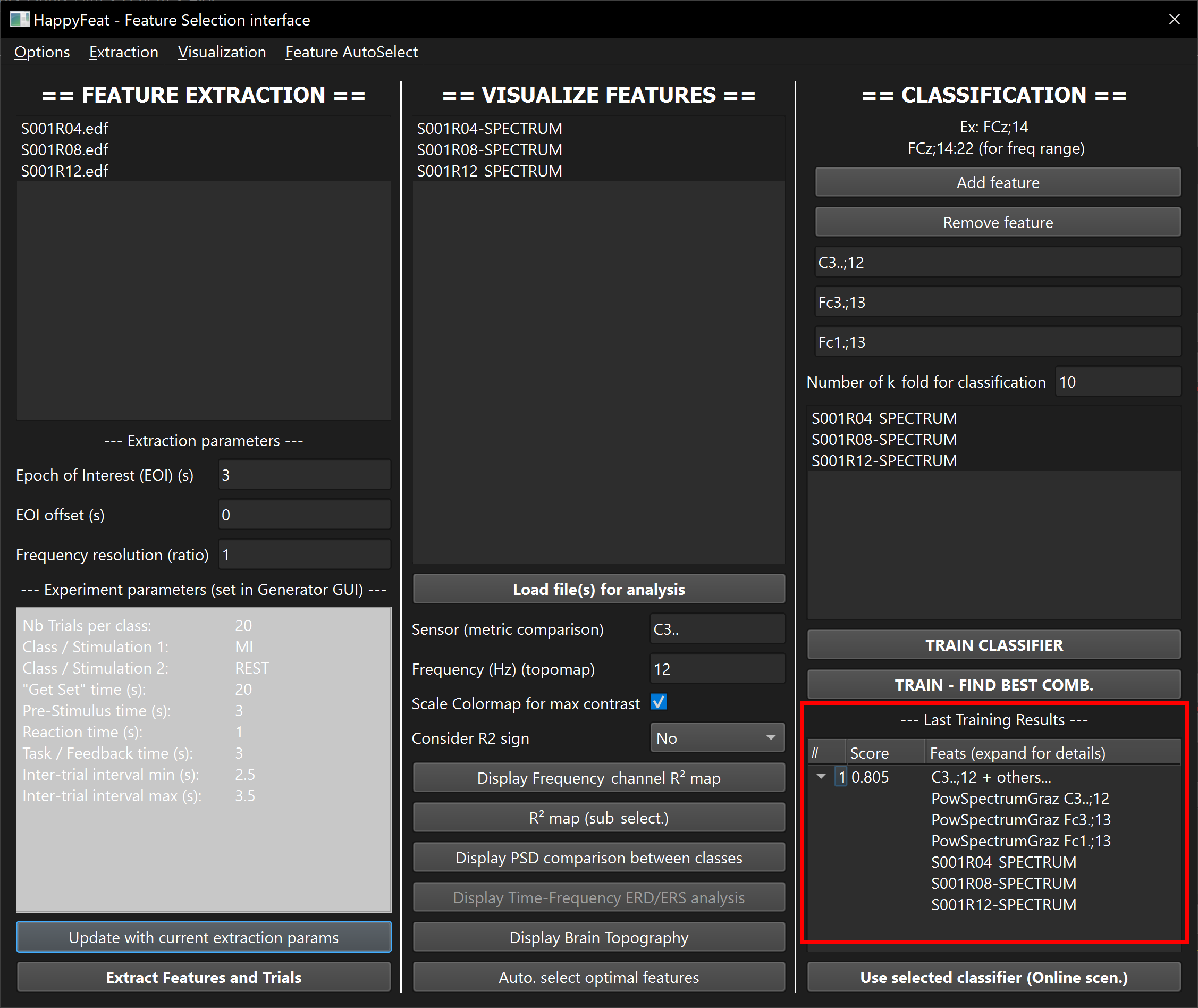
In this tutorial, we will use the second method. Click on Auto. select optimal features. The 3 best features will automatically be selected. Then in the right panel, select all 3 runs in the list, and click on Train Classifier.

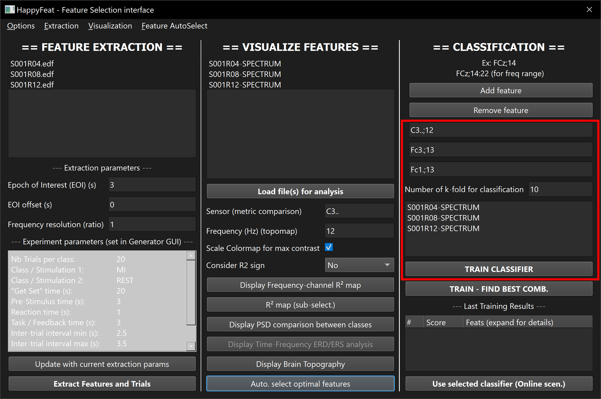
After a few seconds, HappyFeat displays the classification accuracy in a pop-up window. Those results are also available in the lower-right part of the GUI.